After the high of rstudio::conf 2018, I made a (tiny) list of R-related goals for myself:
I need to learn how to use blogdown. Current list of goals: write a package, write a blog post. Let’s call this a...six month list? Lol.
— Larie (@lariebyrd) February 6, 2018
Happily, I was able to knock the second one out back in February, but the first one has taken more work.
The biblionetwork package has just two functions, currently. They are (so creatively named, you guys): make_edgelist : creates edgelists in dataframe format make_nodelist : creates nodelists in dataframe format
I’m not sure if a package already exists out there that performs these functions, but I couldn’t find one when I first started working with co-occurrence lists and networks. I did find a great example from Francois Briatte, which I was able to modify for my work. I’ve since changed the script even further, and benchmarked my various versions to gauge speed: 1
Thanks to this blog post on benchmarking in R (and the “microbenchmark” package), I now know which version of this function is fasterhttps://t.co/6RMfGvO28z #rstats pic.twitter.com/CR4CIOvr0M
— Larie (@lariebyrd) March 14, 2018
Mind you, it’s still not very fast (especially for very large networks, ~104 nodes and >= 106 edges). But it works!
[Update, 2018/03/30 I’m updating this post to use the fivethirtyeight package from Albert, Chester, and Jennifer. Install the package and call the dataset to use it as shown.]
I’m going to walk through it with the “Candy” dataset from FiveThirtyEight. This is a dataset of candy types, with a bunch of variables describing the candies, like “chocolate,” “fruity,” and so on; the full description of the data can be found here in the package reference, and here on the fivethirtyeight data site. We’re going to rework it a little bit and create a network graph of the candies; candy with similar traits should be closer to each other and linked.
# load the data from the fivethirtyeight package

install.packages("fivethirtyeight")
library(fivethirtyeight)

dat <- fivethirtyeight::candy_rankings

# check it out

head(dat)
## # A tibble: 6 x 13
## competitorname chocolate fruity caramel peanutyalmondy nougat
## <chr> <lgl> <lgl> <lgl> <lgl> <lgl>
## 1 100 Grand TRUE FALSE TRUE FALSE FALSE
## 2 3 Musketeers TRUE FALSE FALSE FALSE TRUE
## 3 One dime FALSE FALSE FALSE FALSE FALSE
## 4 One quarter FALSE FALSE FALSE FALSE FALSE
## 5 Air Heads FALSE TRUE FALSE FALSE FALSE
## 6 Almond Joy TRUE FALSE FALSE TRUE FALSE
## # ... with 7 more variables: crispedricewafer <lgl>, hard <lgl>,
## # bar <lgl>, pluribus <lgl>, sugarpercent <dbl>, pricepercent <dbl>,
## # winpercent <dbl>Let’s also remove the “one dime” and “one quarter” entries, because…that’s not food. (They discuss this in the article.)
library(tidyverse)
library(magrittr)

dat %<>%
  filter(!competitorname %in% c("One dime", "One quarter"))

# how many distinct candies are there?
n_distinct(dat$competitorname)
## [1] 83The descriptive columns in the fivethirtyeight package version of this dataset are logical variables - “TRUE” indicating “yes,” this is “chocolate,” and “FALSE” if it is not. We’re going to change this coding a little bit and create text instead. There is probably a more elegant way of doing this, but messing with extracting and looping over colnames is something I don’t want to touch with a long stick, so…
# create new columns with text instead of binary coding

dat_labels <-
  dat %>%
  mutate(choc_lab = ifelse(chocolate, "chocolate", NA),
         fruit_lab = ifelse(fruity, "fruity", NA),
         car_lab = ifelse(caramel, "caramel", NA),
         pea_lab = ifelse(peanutyalmondy,
                                 "peanutyalmondy", NA),
         nou_lab = ifelse(nougat, "nougat", NA),
         crisp_lab = ifelse(crispedricewafer ,
                                   "crispedricewafer", NA),
         hard_lab = ifelse(hard , "hard", NA),
         bar_lab = ifelse(bar, "bar", NA),
         plu_lab = ifelse(pluribus, "pluribus", NA))

# and check

head(dat_labels)
## # A tibble: 6 x 22
## competitorname chocolate fruity caramel peanutyalmondy nougat
## <chr> <lgl> <lgl> <lgl> <lgl> <lgl>
## 1 100 Grand TRUE FALSE TRUE FALSE FALSE
## 2 3 Musketeers TRUE FALSE FALSE FALSE TRUE
## 3 Air Heads FALSE TRUE FALSE FALSE FALSE
## 4 Almond Joy TRUE FALSE FALSE TRUE FALSE
## 5 Baby Ruth TRUE FALSE TRUE TRUE TRUE
## 6 Boston Baked Beans FALSE FALSE FALSE TRUE FALSE
## # ... with 16 more variables: crispedricewafer <lgl>, hard <lgl>,
## # bar <lgl>, pluribus <lgl>, sugarpercent <dbl>, pricepercent <dbl>,
## # winpercent <dbl>, choc_lab <chr>, fruit_lab <chr>, car_lab <chr>,
## # pea_lab <chr>, nou_lab <chr>, crisp_lab <chr>, hard_lab <chr>,
## # bar_lab <chr>, plu_lab <chr>Now! We’re going to reshape this. What we ultimately want is a single descriptor column that has concatenated text. Theoretically, we could use dplyr::unite(), but it doesn’t handle NAs well, so we’ll do it a slightly messier way. We’ll start with dplyr::gather().
# trim columns from dat_labels

dat_labels %<>%
  select(-c(2:13))

# turn to long format, removing NA rows
dat_long <- gather(dat_labels, key = type, value = descriptor, 2:10, na.rm = TRUE) %>%
  select(-type)

# now create a final column that concatenates all candies that share certain descriptors

candy <- aggregate(competitorname ~ descriptor, data = dat_long, paste, collapse = ",")| descriptor | competitorname |
|---|---|
| bar | 100 Grand,3 Musketeers,Almond Joy,Baby Ruth,Charleston Chew,Hershey’s Krackel,Hershey’s Milk Chocolate,Hershey’s Special Dark,Kit Kat,Milky Way,Milky Way Midnight,Milky Way Simply Caramel,Mounds,Mr Good Bar,Nestle Butterfinger,Nestle Crunch,Payday,Snickers,Snickers Crisper,Tootsie Roll Snack Bars,Twix |
| caramel | 100 Grand,Baby Ruth,Caramel Apple Pops,Milk Duds,Milky Way,Milky Way Midnight,Milky Way Simply Caramel,Rolo,Snickers,Snickers Crisper,Sugar Babies,Sugar Daddy,Twix,Werther’s Original Caramel |
| chocolate | 100 Grand,3 Musketeers,Almond Joy,Baby Ruth,Charleston Chew,Hershey’s Kisses,Hershey’s Krackel,Hershey’s Milk Chocolate,Hershey’s Special Dark,Junior Mints,Kit Kat,Peanut butter M&M’s,M&M’s,Milk Duds,Milky Way,Milky Way Midnight,Milky Way Simply Caramel,Mounds,Mr Good Bar,Nestle Butterfinger,Nestle Crunch,Peanut M&Ms,Reese’s Miniatures,Reese’s Peanut Butter cup,Reese’s pieces,Reese’s stuffed with pieces,Rolo,Sixlets,Nestle Smarties,Snickers,Snickers Crisper,Tootsie Pop,Tootsie Roll Juniors,Tootsie Roll Midgies,Tootsie Roll Snack Bars,Twix,Whoppers |
| crispedricewafer | 100 Grand,Hershey’s Krackel,Kit Kat,Nestle Crunch,Snickers Crisper,Twix,Whoppers |
| fruity | Air Heads,Caramel Apple Pops,Chewey Lemonhead Fruit Mix,Chiclets,Dots,Dum Dums,Fruit Chews,Fun Dip,Gobstopper,Haribo Gold Bears,Haribo Sour Bears,Haribo Twin Snakes,Jawbusters,Laffy Taffy,Lemonhead,Lifesavers big ring gummies,Mike & Ike,Nerds,Nik L Nip,Now & Later,Pop Rocks,Red vines,Ring pop,Runts,Skittles original,Skittles wildberry,Smarties candy,Sour Patch Kids,Sour Patch Tricksters,Starburst,Strawberry bon bons,Super Bubble,Swedish Fish,Tootsie Pop,Trolli Sour Bites,Twizzlers,Warheads,Welch’s Fruit Snacks |
| hard | Dum Dums,Fun Dip,Gobstopper,Jawbusters,Lemonhead,Nerds,Pop Rocks,Ring pop,Root Beer Barrels,Runts,Smarties candy,Strawberry bon bons,Tootsie Pop,Warheads,Werther’s Original Caramel |
OKAY. We now have a dataframe that shows, for every candy descriptor, the full list of candies that have that characteristic. E.g., for “chocolate,” it shows: “100 Grand, 3 Musketeers, Almond Joy, Baby Ruth, Charleston Chew (wut?), Hershey’s Krackel, Hershey’s Milk Chocolate,” and so on.
Now we can finally get to more fun stuff. I mean, I guess that was fun. But I’m itching to share my “biblionetwork” package!
It’s hosted on my github:
Install from github and load the package.
# install from github (install_packages("devtools") first if necessary)
devtools::install_github("aczane/biblionetwork")

# load the library
library(biblionetwork)
As I mentioned above, it has two functions: make_nodelist, and make_edgelist. First, we will want to create the nodelist.
# create the list of nodes - this is essentially the list of candies, one per row, in a tidy way.
nodes <- make_nodelist(candy, competitorname, sep = ",")

head(nodes)
## competitorname
## 1 100 Grand
## 2 3 Musketeers
## 3 Air Heads
## 4 Almond Joy
## 5 Baby Ruth
## 6 Boston Baked Beans# and now make the edgelist. This connects nodes that share candy types. This is an undirected network, so edge pairs (i,j) and (j,i) are equivalent.
edges <- make_edgelist(candy, competitorname, sep = ",")
head(edges)## # A tibble: 6 x 3
## X1 X2 weight
## <chr> <chr> <dbl>
## 1 100 Grand 3 Musketeers 2.
## 2 100 Grand Almond Joy 2.
## 3 100 Grand Baby Ruth 3.
## 4 100 Grand Caramel Apple Pops 1.
## 5 100 Grand Charleston Chew 2.
## 6 100 Grand Hershey's Kisses 1.So if two candies share two attributes, they should have an edge weight of two; if they share three attributes, their edge weight should be three.
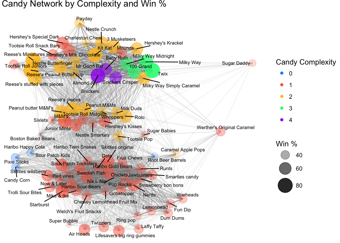
And now, the network graph! We’ll try out tidygraph and ggraph.2
install.packages("tidygraph")
install.packages("thomasp85/ggraph")

library(tidygraph)
library(ggraph)
##
## Attaching package: 'tidygraph'## The following object is masked from 'package:stats':
##
## filterWe’ll want one of the original data columns as a node attribute: winpercent. We also want to make a new attribute, which I’ll just call “complexity:” a scale indicating how many of the descriptors each candy has. That is, if it’s “chocolate” and “peanutyalmondy” and “nougat” (like “Baby Ruth” or “Snickers”, it will have complexity >= 3 (in this case, both are also “caramel”, so it’d be “4.”))
# sum the first six columns of the original dataset: chocolate, fruity, caramel, peanutyalmondy, nougat, crispedricewafer. What is the range?

dat %<>%
  mutate(complexity = chocolate + fruity + caramel + peanutyalmondy + nougat + crispedricewafer)

range(dat$complexity)
## [1] 0 4# join the attributes to the nodes df
nodes <-
nodes %>%
left_join(dat[,c(1,13,14)], by = "competitorname")
# now create the graph object
cg <- tbl_graph(edges = edges, nodes = nodes, directed = FALSE)
summary(cg)## IGRAPH d91ed68 U-W- 83 2024 --
## + attr: competitorname (v/c), winpercent (v/n), complexity (v/n),
## | weight (e/n)cg## # A tbl_graph: 83 nodes and 2024 edges
## #
## # An undirected simple graph with 1 component
## #
## # Node Data: 83 x 3 (active)
## competitorname winpercent complexity
## <chr> <dbl> <int>
## 1 100 Grand 67.0 3
## 2 3 Musketeers 67.6 2
## 3 Air Heads 52.3 1
## 4 Almond Joy 50.3 2
## 5 Baby Ruth 56.9 4
## 6 Boston Baked Beans 23.4 1
## # ... with 77 more rows
## #
## # Edge Data: 2,024 x 3
## from to weight
## <int> <int> <dbl>
## 1 1 2 2.
## 2 1 4 2.
## 3 1 5 3.
## # ... with 2,021 more rowsSo now we have a graph object that has nodes, node attributes (winpercent and complexity), and edges, with edge weights.
So let’s plot this!
# and let's plot

# color scheme
cols <- c("dodgerblue1", "tomato1", "goldenrod1", "springgreen1", "purple")

# now the ggraph
ggraph(cg, layout = 'fr') +
  geom_edge_fan(aes(alpha = weight), edge_colour = "gray54",
                show.legend = FALSE) +
  geom_node_point(aes(size = winpercent, alpha = winpercent,
                      color = as.factor(complexity))) +
  labs(title = "Candy Network by Complexity and Win %") +
  geom_node_text(aes(label = competitorname), size = 2.5,
                 colour = 'black', repel = TRUE,
                 check_overlap = TRUE) +
  scale_alpha_continuous(range = c(0.1, 0.9), name = "Win %") +
  scale_size_continuous(range = c(1,10), name = "Win %") +
  scale_color_manual(name = "Candy Complexity", values = cols) +
  theme_void()
And this is pretty much what you would expect! Similar candies are connected by edges.
The chocolate candy bars are all together, interconnected. Midway through you get chocolate pluribus candies like M&Ms, and then you get into fruitier candies on the other side, which all tend to be pluribus (and erm, where my heart lies). You also see that the fruity candies tend not to be so complex (at least on this scale), but people still like them, whereas the more popular chocolate candies tend to rate higher in complexity.
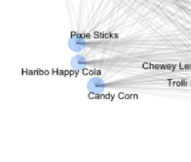
And finally, your reminder that you can’t always trust a simple graph. I love Haribo Happy Cola. But what is it next to?
 CANDY CORN?? THE HORROR.
Anyway, there it is! Let me know if you try out the package and find it helpful, or lacking, or anything at all! For more handy network resources, check out:
- Katya Ognyanova’s website
- Francois Briatte’s curated list of network resources
- Colin Fay’s Gentle Introduction to Network Visualization
Alexej’s post is extremely helpful for benchmarking, btw.↩
For really large networks (104 nodes and >=107 edges), I find
ggnetworkto work a little better, though it requires more tweaking…I’ve gotten the bomb of doom a little too often with tidygraph and ggraph on very large datasets. I’m not sure why this is. I will confess that I haven’t put too much time into it as I have lots of working code written for ggnetwork.↩