I’m Not a Ninja, but I’ve Got Some Slides!

Let’s Get Started

1. Download xaringan. I work in RStudio, so my instructions and example will be specific to this method. You can install it with:

devtools::install_github('yihui/xaringan')

2. To create a new presentation:
   File > New File > R Markdown > From Template > Ninja Presentation

3. This generates a new .Rmd file - it is the .Rmd that creates Yihui’s slide deck. So, if you have the .Rmd open and the slide deck open (or just use the Infinite Moon Reader Add-in and render it in RStudio viewer/html), you can see what code pieces correspond to slide output elements.

4. In the YAML, you would start with the default:

---
title: "Presentation Ninja"
subtitle: "⚔<br/>with xaringan"
author: "Yihui Xie"
date: "2016/12/12"
output:
  xaringan::moon_reader:
    lib_dir: libs
    nature:
      highlightStyle: github
      highlightLines: true
      countIncrementalSlides: false
---

This will format your title slide. I edited it this way:

---
title: "Title Goes Here"
author: "Ariel C. Zane<br/>More Lines Here"
date: "March 2, 2018"
output:
  xaringan::moon_reader:
    # to change color schemes, add this line below
    # to incorporate customized css
    css: ["default", "new-color.css", "default-fonts.css"]
    lib_dir: libs
    nature:
      highlightStyle: github
      highlightLines: true
      countIncrementalSlides: false
---

Here’s the difference:

My understanding is that the default CSS doesn’t explicitly need to be called unless you want to modify it - Yihui gives the explanation here. The “default” .css file appears once you render the .Rmd, along with the default-fonts.css file (some other files also appear: the libs folder and everything in it, and .html output of your .Rmd).

They take effect in this order:
default < new-color.css < default-fonts.css

If you want to overwrite only chunks of it (here, I changed colors in new-color.css, and fonts in default-fonts.css), be mindful of the order. You could also presumably edit the default.css.

I used http://www.color-hex.com to find colors. For my work presentation, I just used basic black and white colors, but here I changed them so that the difference was more marked.¹

Contents of new-color.css:

/*
h1, h2, h3 - font colors for the different headers; removed text shadow
*/

h1, h2, h3 {
  font-weight: normal;
  color: #eb6d13;
  text-shadow: none;
}

/*
for any links
*/

a, a > code {
  color: #eb6d13;
}

/*
highlight color for inline code; 
the rgba takes red, green, blue, alpha arguments
*/
.remark-code-line-highlighted { background-color: rgba(19, 108, 235 0.3); }

/* background color and headers, code, etc., colors for .inverse class slides (e.g., title)
*/

.inverse {
  background-color: #FFFFFF;
}
.inverse, .inverse h1, .inverse h2, .inverse h3, .inverse a, inverse a > code {
  color: #E7165F;
}

5. From here, it’s mostly like working with an R Markdown file. To edit and create your slides, you’ll first want to set your code preferences.

I didn’t set eval = FALSE up here in the overall options because I wanted to run tables that would be included in my code. For later chunks that I didn’t want to be evaluated, I just added eval = FALSE where necessary.²

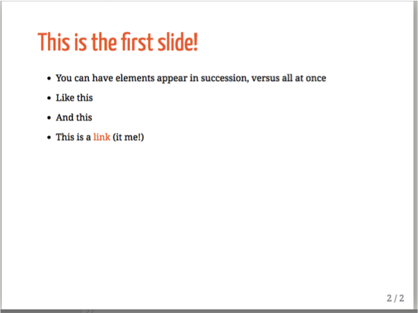
Then you can start with your first (non-title) slide. The syntax is all Pandoc markdown, which you can use the handy R Markdown cheat sheet for:

---
# This is the first slide!

--

- You can have elements appear in succession, versus all at once

--

- Like this

--

- And this

--

- This is a [link](http://tumblr.tastefullyoffensive.com/post/171451780306/squirrel-eats-doughnut#.WpmF52aZOSM) (it me!)

And this is what you would get, ultimately (although each bullet would appear with successive advances - you can see it in the full slide deck at the bottom of the post):

If you want to suppress the message of an evaluated chunk, add message = FALSE:

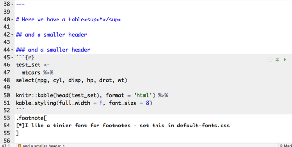
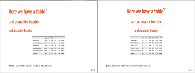
If you want to display tables, use format = ‘html’ in knitr::kable. I also used the kableExtra package to add a little more customization.

test_set <-
  mtcars %>%
  select(mpg, cyl, disp, hp, drat, wt)

knitr::kable(head(test_set), format = 'html') %>%
  kable_styling(full_width = F, font_size = 8)

So the slide .Rmd would look like:

If you wanted to center it, add this to the top:

---
  class: center

And if you want to use the formatting for the title slide (here it doesn’t matter, because all of my backgrounds are white), you would add class: inverse.

We did it!

That’s it! My goal was to help convince you that you could go from 0 to slide deck in a very short amount of time; hopefully this helped. I shared the .html outputs with team members via email; they opened it with a browser and everything worked perfectly. I wasn’t able to save it to pdf from a browser very well, though - it created 8x11 formatted files and didn’t preserve the 4:3 ratio. I looked at some of the documentation about that, but it was the end of the day and I didn’t get very far. If anyone has tips, let me know!

Scroll through the example deck here:³ (source code here)